PID Controller Tuning for Robotic Arms: A Practical Guide

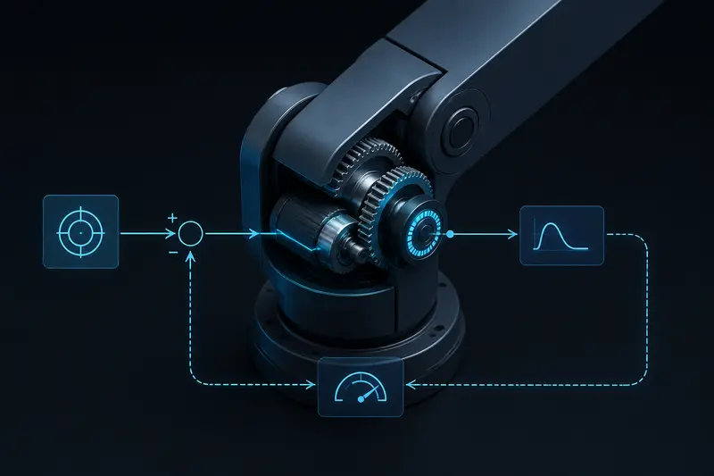
Every robotic arm joint, whether driven by a servo, stepper, or BLDC motor with a closed encoder loop, needs some way to convert a position error into a corrective command. The most common tool for this is the PID controller. PID controller tuning for robotic arms is the process of choosing three gains, proportional, integral, and derivative, so the joint reaches its target quickly, without overshooting, oscillating, or drifting off target under load.

This guide walks through what each term actually does mechanically, two practical tuning methods, and how to recognize and fix the most common tuning mistakes.

What a PID Controller Does in a Robot Joint

A PID controller reads the error between a desired joint position (or velocity) and the measured value from an encoder, then computes a control signal, usually a motor current or PWM duty cycle. The standard continuous-time form is:

u(t) = Kp * e(t) + Ki * ∫ e(t) dt + Kd * de(t)/dt

where e(t) is the position error (setpoint minus measured position). In a discrete control loop running at a fixed rate, this becomes:

error = setpoint - position
integral += error * dt
derivative = (error - last_error) / dt
output = Kp * error + Ki * integral + Kd * derivative
last_error = error

Each term has a distinct mechanical role:

• Proportional (Kp) pushes the joint toward the target in proportion to how far off it is. Too low and the arm feels sluggish and never quite reaches the target under load. Too high and the joint overshoots and oscillates.
• Integral (Ki) accumulates past error over time and eliminates steady-state error, the small residual gap left when Kp alone can't fully counteract gravity or friction. Too much Ki causes slow, growing oscillations known as integral windup.
• Derivative (Kd) reacts to how fast the error is changing, which damps oscillation and reduces overshoot. Too much Kd amplifies encoder noise into jittery, high-frequency motor commands.

Manual Tuning: The Practical Starting Point

For most small to mid-size arm joints, manual tuning is faster than a formal method because you can watch the joint move and react to what you see. The standard sequence is:

1. Set Ki = 0 and Kd = 0. Raise Kp from zero until the joint reaches its target quickly but just starts to overshoot and oscillate slightly.
2. Reduce Kp by roughly 20-30% from that point to leave a margin.
3. Increase Kd gradually. This damps the oscillation from step 1 and lets you push Kp a bit higher again. Stop increasing Kd once you notice the motor buzzing or vibrating, that is encoder noise being amplified.
4. Increase Ki slowly until steady-state error (the joint not quite reaching the exact target under a static load, like an arm holding a weight against gravity) disappears. Watch for slow oscillations developing, a sign Ki is too high.

A joint holding position against gravity is the best test case, since gravity creates a constant disturbance torque that only integral action can fully cancel. If your arm sags slightly under a payload with Kp and Kd tuned well, that gap is exactly what Ki is for.

Ziegler-Nichols: A Structured Alternative

When manual tuning feels too trial-and-error, the Ziegler-Nichols method gives a repeatable procedure:

1. Set Ki = 0 and Kd = 0.
2. Increase Kp until the joint oscillates continuously at a constant amplitude, neither growing nor shrinking. Record this gain as the ultimate gain Ku, and measure the oscillation period Tu in seconds.
3. Compute the gains from the classic Ziegler-Nichols table:

• Kp = 0.6 * Ku
• Ki = 1.2 * Ku / Tu
• Kd = 0.075 * Ku * Tu

Ziegler-Nichols tends to produce a fairly aggressive, somewhat oscillatory response, which is a reasonable starting point but usually benefits from manual fine-tuning afterward, particularly reducing Kp by 10-20% for a joint carrying a variable payload.

Common Failure Modes and Fixes

Overshoot and Ringing

The joint passes the target and oscillates before settling. This is almost always Kp too high relative to Kd. Reduce Kp, or increase Kd to add damping, but watch for noise amplification if Kd climbs too far.

Steady-State Error Under Load

The joint settles just short of or past the target when holding a static load. This is the textbook symptom of insufficient Ki. Add a small amount of integral gain, and consider a feedforward gravity compensation term if the payload varies significantly, since a large Ki to fight a large, predictable disturbance also makes the loop more prone to windup.

Integral Windup

If the joint is mechanically blocked or the error stays large for a long period, the integral term can accumulate an enormous value, causing a large overshoot once the obstruction clears. Clamp the integral term to a maximum value (anti-windup clamping), or freeze integration whenever the output is saturated.

High-Frequency Jitter

A buzzing or vibrating joint at standstill usually means Kd is amplifying encoder quantization noise. Lowering Kd, or low-pass filtering the derivative term before applying the gain, usually resolves this without sacrificing much damping.

Tuning Per Joint, Not Per Arm

A common mistake is applying one set of PID gains to every joint in a multi-DOF arm. Each joint carries a different effective inertia, depending on the mass and length of the links it moves, so a base joint supporting the whole arm needs different gains than a wrist joint moving only the end effector. Tune each joint independently, ideally with the arm in a few representative poses, since gravity loading on a joint changes with arm configuration.

If your control loop also handles multi-joint coordination, note that PID tuning happens at the single-joint level, well below trajectory planning. Getting the low-level loop stable and accurate first makes any higher-level trajectory planning far more predictable, since the planner can then assume each joint actually tracks the commands it's given.

Summary

PID controller tuning for robotic arms comes down to matching Kp, Ki, and Kd to the specific inertia, friction, and disturbance profile of each joint. Start with Kp for responsiveness, add Kd for damping, and finish with a small Ki to eliminate steady-state error, watching for windup and noise amplification along the way. Whether you tune manually or with Ziegler-Nichols as a starting point, always validate under the actual payload and pose the joint will operate in, since gains tuned on an unloaded arm rarely hold up once a gripper is carrying real weight.