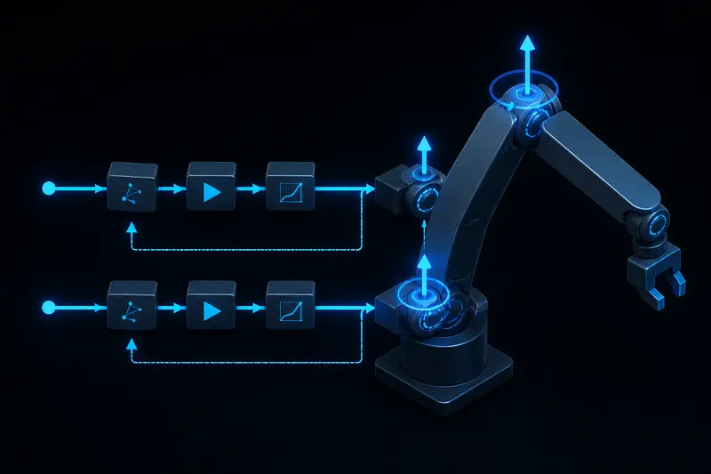
Computed Torque Control for Robot Arms: A Worked Numeric Example

Computed torque control is a way to make a robot arm's tracking error behave like a plain double integrator, no matter how nonlinear the arm's real dynamics are. Instead of tuning a PID loop against a moving, coupled, gravity-loaded plant and hoping the gains hold up everywhere in the workspace, computed torque control cancels the arm's actual dynamics with a model of those same dynamics, then closes a simple linear loop on top. This article works through the full derivation and a numeric example for a two-link arm, so you can check your own implementation's torque output against a known-good number.

Why computed torque control matters

A robot arm's equation of motion is usually written as:

M(q) * qddot + C(q, qdot) * qdot + G(q) = tau

where q is the joint angle vector, M(q) is the (configuration-dependent) inertia matrix, C(q, qdot) collects the Coriolis and centrifugal terms, G(q) is the gravity torque vector, and tau is the vector of commanded joint torques. If you have already added a gravity feedforward term to a PD loop, you have handled G(q) alone. Computed torque control goes further: it cancels M(q) and C(q, qdot) as well, using the arm's own inverse dynamics model.

The controller sets:

tau = M(q) * (qddot_desired + Kd * e_dot + Kp * e) + C(q, qdot) * qdot + G(q)

where e = q_desired - q is the tracking error. Substitute this back into the equation of motion (assuming a perfect model, so the M(q) terms cancel) and the closed-loop error dynamics collapse to:

e_ddot + Kd * e_dot + Kp * e = 0

That is a linear, decoupled second-order system in each joint, exactly the same form as a mass-spring-damper. You pick Kp and Kd the same way you would tune a PD loop on a unit-mass system, and the tracking behavior is uniform across the whole workspace instead of degrading near singularities or heavy configurations.

Building the two-link model

Take a two-link planar arm in a vertical plane (so gravity acts on both links), with:

• Link 1: mass m1 = 2.0 kg, length l1 = 0.35 m, center of mass at l1/2, moment of inertia about its own center I1 = 0.03 kg*m^2
• Link 2: mass m2 = 1.2 kg, length l2 = 0.30 m, center of mass at l2/2, moment of inertia about its own center I2 = 0.01 kg*m^2
• Joint angles q1 = 30 deg, q2 = 45 deg, with q2 measured relative to link 1

The standard two-link inertia matrix entries are:

M11 = I1 + I2 + m1*(l1/2)^2 + m2*(l1^2 + (l2/2)^2 + 2*l1*(l2/2)*cos(q2)) M12 = M21 = I2 + m2*((l2/2)^2 + l1*(l2/2)*cos(q2)) M22 = I2 + m2*(l2/2)^2

Plugging in numbers (cos(45 deg) = 0.7071):

M11 = 0.03 + 0.01 + 2.0*(0.175)^2 + 1.2*(0.35^2 + 0.15^2 + 2*0.35*0.15*0.7071) = 0.03 + 0.01 + 0.0613 + 1.2*(0.1225 + 0.0225 + 0.0742) = 0.1013 + 1.2*0.2192 = 0.1013 + 0.2630 = 0.3643 kg*m^2 M12 = 0.01 + 1.2*(0.0225 + 0.35*0.15*0.7071) = 0.01 + 1.2*(0.0225 + 0.0371) = 0.01 + 0.0715 = 0.0815 kg*m^2 M22 = 0.01 + 1.2*0.0225 = 0.01 + 0.027 = 0.037 kg*m^2

The Coriolis/centrifugal term for this arm reduces to a single coefficient h = -m2 * l1 * (l2/2) * sin(q2), giving:

C(q, qdot) * qdot = [ h*qdot2*(2*qdot1 + qdot2), -h*qdot1^2 ] h = -1.2 * 0.35 * 0.15 * sin(45 deg) = -1.2*0.35*0.15*0.7071 = -0.0446

At a moderate motion state, qdot1 = 0.5 rad/s and qdot2 = 0.3 rad/s, this evaluates to:

C*qdot row 1 = -0.0446 * 0.3 * (2*0.5 + 0.3) = -0.0446*0.3*1.3 = -0.0174 N*m C*qdot row 2 = -(-0.0446) * 0.5^2 = 0.0446*0.25 = 0.0112 N*m

And the gravity vector, using g = 9.81 m/s^2:

G1 = (m1*(l1/2) + m2*l1)*g*cos(q1) + m2*(l2/2)*g*cos(q1+q2) G2 = m2*(l2/2)*g*cos(q1+q2)

With q1+q2 = 75 deg (cos = 0.2588) and q1 = 30 deg (cos = 0.8660):

G1 = (2.0*0.175 + 1.2*0.35)*9.81*0.8660 + 1.2*0.15*9.81*0.2588 = (0.35 + 0.42)*9.81*0.8660 + 1.766*0.2588 = 0.77*8.4966 + 0.457 = 6.542 + 0.457 = 6.999 N*m G2 = 1.2*0.15*9.81*0.2588 = 1.766*0.2588 = 0.457 N*m

Computing the commanded torque

Suppose the desired trajectory calls for qddot_desired = [0.2, 0.1] rad/s^2 at this instant, and the current tracking error is small: e = [0.01, -0.005] rad, e_dot = [0.02, -0.01] rad/s. Choose Kp = 100 and Kd = 20 for both joints (a critically-damped-ish choice for a unit-mass double integrator; the actual damping ratio here is Kd / (2*sqrt(Kp)) = 20/20 = 1.0, so this is exactly critically damped).

The linear correction term per joint is:

u1 = qddot_desired1 + Kd*e_dot1 + Kp*e1 = 0.2 + 20*0.02 + 100*0.01 = 0.2 + 0.4 + 1.0 = 1.6 rad/s^2 u2 = qddot_desired2 + Kd*e_dot2 + Kp*e2 = 0.1 + 20*(-0.01) + 100*(-0.005) = 0.1 - 0.2 - 0.5 = -0.6 rad/s^2

Now apply M(q) * u:

tau1_inertial = M11*u1 + M12*u2 = 0.3643*1.6 + 0.0815*(-0.6) = 0.5829 - 0.0489 = 0.534 N*m tau2_inertial = M21*u1 + M22*u2 = 0.0815*1.6 + 0.037*(-0.6) = 0.1304 - 0.0222 = 0.1082 N*m

Add back the Coriolis and gravity terms computed above:

tau1 = 0.534 + (-0.0174) + 6.999 = 7.516 N*m tau2 = 0.1082 + 0.0112 + 0.457 = 0.5764 N*m

Notice how the gravity term dominates both joints at this pose, exactly as it would in a pure gravity-compensation scheme, but the inertial and Coriolis corrections are now baked in automatically instead of being left for a generic PD gain to fight. If you commanded only Kp*e + Kd*e_dot without the inverse dynamics terms, the arm would need much higher gains to track the same trajectory, and those gains would need to change as the arm's configuration (and therefore M(q)) changes.

Where computed torque control breaks down

• Model accuracy. The cancellation only works as well as your M(q), C(q,qdot), and G(q) estimates. Errors in mass, center-of-mass location, or unmodeled friction leave residual dynamics that the linear Kp/Kd loop still has to absorb.
• Computation rate. Every control cycle needs a fresh inverse dynamics evaluation, which is more expensive than a PID update. This ties directly into loop timing budget decisions: if your loop rate can't sustain the extra computation without introducing jitter, the model-based benefit can be outweighed by timing error.
• Torque saturation. The computed torque can exceed what the actuator can deliver, especially near full extension where gravity torque is largest. Clamping tau without accounting for the mismatch reintroduces nonlinear error the linear design assumed away.

In practice, computed torque control is most worth the added complexity on arms with well-characterized mass properties and a control loop fast enough to run the inverse dynamics every cycle without eating into the timing margin. For lighter, less precisely modeled arms, a PD loop with a gravity feedforward term is often close enough, and considerably simpler to implement and debug.