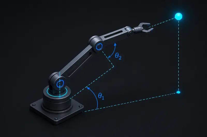
Inverse Kinematics Explained: How Robotic Arms Solve for Joint Angles

Inverse kinematics explained simply: it is the math a robotic arm uses to figure out which joint angles will place its end effector at a specific position and orientation. You tell the arm where you want the gripper to be, and inverse kinematics tells the motors how far to rotate to get it there. This is the opposite problem of forward kinematics, which starts from known joint angles and computes where the end effector ends up.

Forward kinematics is straightforward: chain a series of rotation and translation matrices together, one per joint, and you get the end-effector pose. Inverse kinematics inverts that chain, and that inversion is where things get mathematically messy.

Why inverse kinematics is harder than forward kinematics

Forward kinematics is a single deterministic function: one set of joint angles always produces exactly one end-effector pose. Inverse kinematics is not so clean, for three reasons.

• Multiple solutions. A 6-DOF arm can often reach the same point with its elbow up or elbow down, or with the wrist rotated a different way. There can be zero, one, or infinitely many valid joint configurations for a single target.
• Unreachable targets. If the target lies outside the arm's workspace, no solution exists at all. The solver has to detect this rather than return garbage.
• Nonlinear equations. The forward kinematics chain is full of sines and cosines of joint angles, so solving it backward means solving a system of nonlinear equations, not a simple linear inverse.

Analytical (closed-form) solutions

For simple arms, usually 2 or 3 DOF operating in a plane, you can derive an exact formula using trigonometry. Consider a 2-link planar arm with link lengths L1 and L2, base at the origin, and target point (x, y). The angle at the elbow comes from the law of cosines:

d2 = x*x + y*y
cos_theta2 = (d2 - L1*L1 - L2*L2) / (2 * L1 * L2)
theta2 = acos(cos_theta2)          # elbow angle, +/- for elbow-up or elbow-down

k1 = L1 + L2 * cos(theta2)
k2 = L2 * sin(theta2)
theta1 = atan2(y, x) - atan2(k2, k1)   # shoulder angle

This gives you both elbow-up and elbow-down solutions depending on the sign you choose for theta2. Closed-form solutions like this are fast, exact, and cheap enough to run at full control-loop rate, which is why they are still used for simple pick-and-place arms and for the wrist sub-chain of larger manipulators. The catch is that deriving them by hand only stays practical up to about 3 DOF; beyond that the algebra becomes unmanageable.

Jacobian-based numerical methods

For arms with more joints, the standard approach is iterative and uses the manipulator Jacobian, a matrix that relates small changes in joint angles to small changes in end-effector position and orientation:

delta_x = J(theta) * delta_theta

To move toward a target, you invert this relationship at each iteration:

error = target_pose - current_pose
delta_theta = J_pseudo_inverse(theta) * error
theta = theta + step_size * delta_theta

You recompute the Jacobian, take a small step, check the new error, and repeat until the end effector converges on the target. Since a true inverse only exists for a square, non-singular Jacobian, most implementations use the Moore-Penrose pseudoinverse or a damped least-squares version (often called Damped Least Squares or Levenberg-Marquardt IK) to stay stable near singularities, where the arm loses a degree of freedom in some direction and the Jacobian becomes ill-conditioned.

This is the general-purpose workhorse behind IK solvers in ROS2's MoveIt, in most robot simulators, and in animation rigs. It handles arbitrary DOF counts and redundant arms, at the cost of needing several iterations per solve and a reasonable initial guess to converge on the right local solution.

CCD and FABRIK: lightweight alternatives

Cyclic Coordinate Descent (CCD) skips the Jacobian entirely. It works backward from the end effector, adjusting one joint at a time to reduce the distance to the target, then moves to the next joint up the chain and repeats. It is simple to implement and cheap per iteration, though it can produce less natural-looking joint configurations than Jacobian methods.

FABRIK (Forward And Backward Reaching Inverse Kinematics) treats the arm as a chain of rigid segments and repositions joints along straight lines toward the target in a forward pass, then a backward pass back to the fixed base, iterating until the chain satisfies both the target and the fixed base constraint. It avoids matrix inversion altogether and tends to converge in very few iterations for chain-like structures, which makes it popular in game character rigs and some low-power embedded arms.

Practical considerations when implementing inverse kinematics

• Joint limits. A mathematically valid solution can still be physically impossible if it requires a joint to rotate past its mechanical stop. Clamp or reject solutions that violate limits.
• Singularities. Near full arm extension or certain wrist orientations, small Cartesian movements can require very large joint velocities. Damped least-squares Jacobian methods handle this more gracefully than a plain pseudoinverse.
• Solution selection. When multiple valid configurations exist, pick the one closest to the arm's current joint angles to avoid sudden, large movements between control cycles.
• Orientation, not just position. Full 6-DOF IK needs to match both end-effector position and orientation, which roughly doubles the number of constraints the solver must satisfy compared to a position-only solve.

If you are tuning the resulting joint controllers after your IK solver produces target angles, the underlying position loop is typically still a standard PID controller, so getting that loop well tuned matters just as much as getting the kinematics right.

Choosing an approach

For a 2 or 3 DOF arm confined to a plane, derive the closed-form solution: it is exact and fast enough for any control loop. For a general-purpose serial arm with 5 or more DOF, reach for a Jacobian-based numerical solver, since libraries like KDL, TRAC-IK, and MoveIt already implement damped least-squares IK you can call directly. For character animation or very low-power embedded chains where matrix math is expensive, CCD or FABRIK are lighter alternatives that trade some solution quality for simplicity.