LQR Control for Robot Arms: A Practical Introduction

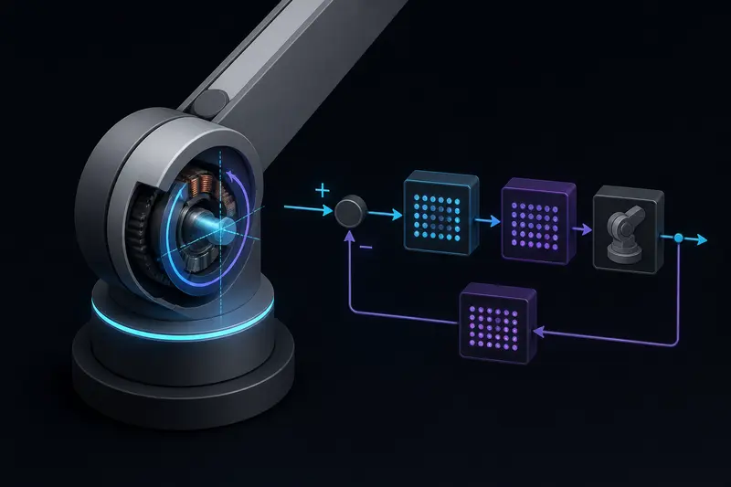
If you have already tuned a PID controller for a robot arm joint, you know the limits well: three gains, a lot of trial and error, and a controller that only really knows about the error on that one joint. LQR control for robot arms takes a different approach. Instead of reacting to error, it uses a full model of the joint's dynamics and a cost function to compute the mathematically optimal feedback gains for every state at once. This article works through the state-space setup, the Q/R tuning process, and a direct comparison against a tuned PID loop on the same joint.

Why move past PID for robot arm control

A PID controller only sees one number: the position error. It has no idea what the velocity is doing except through its own derivative term, and it has no model of the joint's inertia, damping, or gear ratio. That works fine for a single, well-isolated joint with a stiff gearbox. It works less well when:

• Joint dynamics are lightly damped, so overshoot and ringing are hard to remove without slowing the response.
• The controller needs to reject an external disturbance (a payload change, a cable snag) predictably rather than just eventually.
• You want a repeatable, less trial-and-error way to hit a target bandwidth and damping ratio.

LQR (Linear Quadratic Regulator) control replaces manual gain guessing with an optimization problem: given a linear model of the system and a cost function that penalizes state error and control effort, solve for the feedback gain matrix that minimizes that cost over all time. The result is full-state feedback, not just error feedback.

Building the state-space model of a robot joint

Start with a single revolute joint driven by a DC motor through a gearbox, modeled as a second-order system: angle theta, angular velocity omega, with viscous damping b and effective inertia J (motor plus reflected load inertia through the gear ratio). The equation of motion is:

J * theta_ddot + b * theta_dot = tau

where tau is the motor torque at the joint. Define the state vector x = [theta, omega]^T and the input u = tau. In state-space form:

x_dot = A*x + B*u

with:

A = [[0, 1],
     [0, -b/J]]

B = [[0],
     [1/J]]

As a concrete example, take a joint with J = 0.02 kg*m^2 (motor plus reflected load inertia) and b = 0.1 N*m*s/rad. Then:

A = [[0, 1],
     [0, -5.0]]

B = [[0],
     [50.0]]

This is the same physical joint you would tune a PID loop for, just written in a form LQR can use directly. Note that A and B come from real, measurable quantities: J from the datasheet (or a swing-down test), b from a similar swing-down decay measurement, and the gear ratio squared multiplying the reflected load inertia.

Setting up the cost function: Q and R

LQR minimizes a cost function of the form:

J_cost = integral of (x^T * Q * x + u^T * R * u) dt

Q is a matrix that penalizes state error, and R penalizes control effort. For a single joint with state [theta, omega], a diagonal Q is the natural starting point:

Q = [[q1, 0],
     [0, q2]]

R = [[r1]]

The ratio between Q and R is what matters, not their absolute scale. A practical starting point:

• Set q1 (position weight) high if position accuracy matters most, for example q1 = 100.
• Set q2 (velocity weight) lower, for example q2 = 1, unless velocity overshoot itself is a problem (e.g. a joint near a mechanical limit).
• Set r1 to reflect actuator cost. A small r1 (like 0.01) allows aggressive torque commands and gives a fast, stiff response. A larger r1 (like 1.0) produces a gentler response that uses less peak torque, useful if you are close to motor current limits.

In practice you sweep these values rather than deriving them analytically. A reasonable workflow: fix R, start with Q as the identity matrix, solve, simulate the step response, then scale q1 up if the response is too slow, or scale r1 up if commanded torque is unrealistically high for your motor.

Solving for the gain matrix

LQR reduces to solving the continuous-time algebraic Riccati equation for a matrix P:

A^T*P + P*A - P*B*R^-1*B^T*P + Q = 0

and then computing the optimal gain:

K = R^-1 * B^T * P

The control law is then simply u = -K*x, full-state feedback rather than error-only feedback. You do not solve the Riccati equation by hand; every major numerical library has a solver. In Python with SciPy:

import numpy as np
from scipy.linalg import solve_continuous_are

A = np.array([[0, 1], [0, -5.0]])
B = np.array([[0], [50.0]])
Q = np.diag([100, 1])
R = np.array([[0.01]])

P = solve_continuous_are(A, B, Q, R)
K = np.linalg.inv(R) @ B.T @ P
print(K)  # e.g. K = [[100.0, 4.47]]

The resulting K gives you two gains: one on position error, one on velocity. Unlike PID, there is no separate integral term by default. If you need zero steady-state error under a constant disturbance (like gravity loading on a non-horizontal joint), augment the state with the integral of position error and re-solve, which is the same trick used in gain-scheduled and LQI (linear quadratic integral) designs.

LQR vs PID on the same joint: what changes

Running both controllers on the same simulated joint (same J, same b, same actuator torque limit) highlights the practical differences rather than a purely theoretical one:

• Tuning process: PID tuning is iterative and manual (Ziegler-Nichols or hand-tuning three coupled gains). LQR tuning is choosing two or three cost weights, then letting the Riccati solver compute the gains directly. Retuning after a design change (say, a different gear ratio) means recomputing A and B and re-solving, not re-guessing gains from scratch.
• Response shape: A well-tuned PID and a well-tuned LQR controller can produce very similar step responses on a simple single joint like this one. The practical gap opens up on coupled or higher-order systems.
• Disturbance handling: Because LQR uses full-state feedback, it reacts to velocity disturbances (not just position error) immediately, which tends to damp out disturbances like a bumped joint faster than PID's derivative term, which is acting on a noisier estimate of the same information.
• Multi-joint coupling: This is where LQR earns its complexity. For a multi-DOF arm where joint torques couple through the manipulator's inertia matrix, you can build a combined state-space model across all joints and get one LQR gain matrix that accounts for that coupling. PID loops per joint have no way to represent that coupling at all; each loop is blind to what the other joints are doing.
• Computational cost: PID is three multiplies and an add, trivial on any microcontroller. LQR is one matrix-vector multiply per control cycle once K is computed offline, which is also cheap at runtime, but the offline Riccati solve requires more than a microcontroller can reasonably do live, so K is normally computed on a workstation and hardcoded or updated at a much slower rate.

When to actually use LQR on a robot arm

For a single, well-isolated joint with a stiff gearbox and no significant coupling to other joints, a tuned PID controller (see our PID tuning guide) is often good enough and much simpler to implement and debug. LQR earns its added complexity when:

• You have a validated dynamic model (from CAD-derived inertias or system identification), since LQR performance is only as good as A and B.
• Multiple joints interact mechanically and you want one controller that accounts for that coupling.
• You need predictable, tunable disturbance rejection rather than trial-and-error gain adjustment.

If you do not have a trustworthy model of J and b, LQR will compute gains that are optimal for the wrong system, which is worse than a hand-tuned PID loop that was tuned against the real hardware directly. Model quality, not the control law, is usually the limiting factor in practice.