Sensorless BLDC Motor Commutation: A Worked Back-EMF Zero-Crossing Timing Example

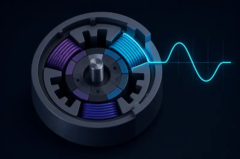
Sensored BLDC commutation reads three hall sensors and looks up the next phase state in a table. Sensorless BLDC motor commutation throws the hall sensors away and infers rotor position from the motor's own electrical behavior instead: at any instant, one of the three phases is left unenergized (floating), and that floating phase still shows a voltage induced by the rotor magnets sweeping past it. That induced voltage is the back-EMF, and the moment it crosses the motor's electrical midpoint is a reliable, fixed marker of rotor position. Most guides stop at "detect the zero crossing, then wait 30 electrical degrees before commutating." This article works through what that wait actually costs in microseconds, why it changes every commutation step, and where the whole scheme falls apart at low speed.

What back-EMF zero-crossing detection actually measures

In six-step (trapezoidal) commutation, only two of the three phases are driven at any time; the third is floating. As the rotor's permanent magnets sweep past that floating winding, they induce a back-EMF voltage in it proportional to rotor speed. For an ideally wound trapezoidal BLDC motor, that floating-phase voltage crosses the electrical midpoint (roughly half the bus voltage, referenced through a resistor divider) exactly once per 60-degree commutation sector, at the point 90 electrical degrees away from the sector's start and 30 electrical degrees before the next commutation event is due.

So the control loop is simple in principle: watch the floating phase's voltage, compare it against the midpoint reference with a comparator or ADC, latch the moment it crosses, then commutate to the next step exactly 30 electrical degrees later. The entire scheme hinges on that 30-degree delay being timed correctly, and that delay is not a fixed number, it depends on how fast the motor is currently spinning.

The worked example: turning 30 degrees into microseconds

Take a small robot wheel-hub BLDC motor with 4 pole pairs (8 magnet poles), spinning at 3000 mechanical RPM. First convert mechanical speed to electrical frequency, since commutation timing lives entirely in the electrical domain:

mechanical_rev_per_sec = 3000 / 60 = 50 rev/s
electrical_freq_Hz = mechanical_rev_per_sec * pole_pairs
electrical_freq_Hz = 50 * 4 = 200 Hz

One full electrical cycle (360 electrical degrees) takes:

electrical_period_us = 1,000,000 / electrical_freq_Hz
electrical_period_us = 1,000,000 / 200 = 5000 us

The 30-degree delay after a zero crossing is then a fixed fraction of that period:

delay_us = electrical_period_us * (30 / 360)
delay_us = 5000 * 0.0833 = 416.7 us

At 3000 RPM with this motor, the controller waits roughly 417 microseconds after each detected zero crossing before switching to the next commutation step. Now double the speed to 6000 RPM and redo the same three lines: electrical frequency becomes 400 Hz, the electrical period halves to 2500 us, and the delay halves to about 208 microseconds. Halve the speed to 1500 RPM instead and the delay doubles to roughly 833 microseconds. The delay is inversely proportional to speed, which is the whole reason a fixed-microsecond delay constant does not work for sensorless BLDC control across any real speed range: it has to be recomputed from the time between the last two zero crossings (or the last two commutation events), every single step.

Why the timer has to be adaptive, not a lookup constant

In practice, firmware measures the time between consecutive commutation events (call it T_step, nominally one sixth of the electrical period) using a hardware timer, then arms the next commutation to fire at T_step / 2 after the most recent zero crossing, since the crossing falls at the midpoint of a commutation step for an idealized trapezoidal back-EMF waveform. This is effectively a simple phase-locked loop: each new T_step measurement updates the estimate used for the next delay, so the commutation timing tracks acceleration and deceleration instead of assuming constant speed. A motor accelerating quickly under load will have its most recent T_step measurement run slightly stale by the time it is used, which is one source of the commutation timing error that shows up as extra current draw and audible noise during hard accelerations, distinct from the six-step torque ripple inherent to trapezoidal drive discussed in hall sensor commutation.

The low-speed blind spot: blanking time and weak back-EMF

The zero-crossing scheme has two compounding problems at low speed, and both come from the same physics: back-EMF amplitude is proportional to rotor speed. Below some threshold, usually a few percent of rated RPM, the signal becomes too weak relative to switching noise to detect reliably at all. That is the well-known reason sensorless BLDC controllers cannot start from a dead stop using zero-crossing detection and instead use an open-loop "align and go" ramp: force a fixed commutation sequence at increasing frequency for a short startup period, building enough speed for a usable back-EMF signal, then hand off to closed-loop zero-crossing detection once a few consecutive valid crossings are seen.

The second problem is PWM demagnetization (blanking) time. Every time a phase switches, the freewheeling diode current and winding inductance produce ringing on the floating phase for a short window after each PWM edge, large enough to trigger false zero crossings if sampled during that window. Firmware handles this by blanking, ignoring the floating-phase reading for a fixed window after every PWM transition, typically tens of microseconds. Compare that blanking window against the worked numbers above: at 3000 RPM the entire delay-to-commutation window is only about 417 microseconds, so a 50-microsecond blanking window consumes over 10 percent of the available detection time. At low speed the ratio gets worse in the wrong direction, since the electrical period stretches out but the blanking window (tied to switching transients, not electrical speed) stays roughly constant, which is why sensorless zero-crossing detection becomes unreliable well before the back-EMF signal itself vanishes entirely.

Practical implications for a robot joint or wheel motor

• Sensorless commutation removes hall sensor wiring and cost, which matters for a small mobile robot wheel motor, but it costs you low-speed control authority, which matters more for a robot arm joint that needs precise slow-speed positioning.
• If your application spends significant time below roughly 10 percent of rated RPM, for example a robot arm joint holding a slow pose, plan for a hall sensor, encoder, or hybrid startup ramp instead of relying on zero-crossing detection down to zero speed.
• When debugging jittery or stalling sensorless commutation, check the actual computed delay against your PWM blanking time at the speeds where it fails, using the same period and delay calculation shown above, before assuming the comparator threshold or filtering is wrong.

Conclusion

Sensorless back-EMF commutation is not magic, it is a timing problem with a clean closed-form answer: electrical frequency from pole-pair count and RPM, electrical period from frequency, and a 30-degree delay that is a fixed fraction of that period recomputed every step. The scheme's real limits show up doing that same arithmetic at low speed, where the fixed blanking window starts eating a large fraction of an electrical period that has grown long, and where a weakening back-EMF signal runs into switching noise. Knowing the actual numbers, not just the qualitative "detect the crossing, wait 30 degrees" description, is what tells you whether sensorless control is even a reasonable choice for your specific joint or wheel motor's speed range.