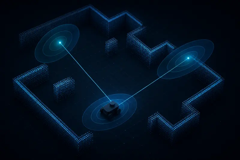
EKF-SLAM explained the way most tutorials do it stops at the symbolic equations: state vector x, covariance P, Jacobians F and H, Kalman gain K. That notation is correct, but it hides what actually happens to the numbers. This article walks through one full predict-update cycle with real values, so you can see exactly how a robot's uncertainty about its own pose and about landmark positions shrinks after a single measurement.
What EKF-SLAM Actually Estimates
In plain SLAM, you either know the map and estimate the robot's pose (localization), or you know the pose and build the map. In real SLAM you know neither exactly, so EKF-SLAM estimates both at once by putting them in a single joint state vector:
x = [ x_r, y_r, theta_r, x_l1, y_l1, x_l2, y_l2, ... ]^TThe first three entries are the robot pose (position and heading). Every pair after that is one landmark's position in the world frame. The joint covariance matrix P is square with the same dimension as x, and its off-diagonal blocks are the key to SLAM: they encode the correlation between robot pose error and landmark position error. When the robot re-observes a landmark it already mapped, those correlations let the update correct the robot's pose and tighten the landmark's uncertainty simultaneously.
Our Concrete Setup
Take a differential-drive robot (see our differential drive kinematics article for how wheel odometry produces the motion estimate below) that has already mapped one landmark and is about to observe it again after a short move. To keep the arithmetic tractable by hand, we use a state with the robot pose plus one landmark:
x = [x_r, y_r, theta_r, x_l, y_l]^TBefore the move, the filter's belief is:
x = [0.00, 0.00, 0.00, 5.00, 2.00]^T   (meters, radians)

P = [ 0.010  0      0      0      0
      0      0.010  0      0      0
      0      0      0.005  0      0
      0      0      0      0.20   0
      0      0      0      0      0.20 ]
The robot is fairly confident about itself (variance 0.01 m^2 in x and y, 0.005 rad^2 in heading) and moderately confident about the landmark (variance 0.20 m^2 in each axis, since it was only observed once before).
Step 1: Prediction from Odometry
Wheel odometry reports a motion of delta_x = 1.00 m forward and delta_theta = 0.10 rad turn, giving a simple prediction for the robot pose (landmarks do not move, so their predicted state is unchanged):
x_r' = x_r + delta_x * cos(theta_r) = 0.00 + 1.00 * cos(0) = 1.00
y_r' = y_r + delta_x * sin(theta_r) = 0.00 + 1.00 * sin(0) = 0.00
theta_r' = theta_r + delta_theta   = 0.00 + 0.10           = 0.10

x_predicted = [1.00, 0.00, 0.10, 5.00, 2.00]^T
The motion Jacobian F with respect to the robot pose (landmark rows/columns are identity since landmarks are static) is:
F_x = [ 1  0  -delta_x*sin(theta_r)
        0  1   delta_x*cos(theta_r)
        0  0   1                    ]
    = [ 1  0   0.00
        0  1   1.00
        0  0   1                    ]
Process noise from wheel slip and odometry error adds Q = diag(0.02, 0.02, 0.01) to the robot-pose block only. Propagating the covariance (P' = F P F^T + Q, with F extended by identity for the landmark rows) gives an updated robot-pose block:
P_rr' = [ 0.030  0      0
          0      0.040  0.010
          0      0.010  0.015 ]
Notice the off-diagonal 0.010 term between y and theta: turning while moving couples heading uncertainty into y-position uncertainty. This is the kind of correlation a diagonal-only "just track x, y, theta separately" approach would silently lose.
Step 2: The Measurement
After the move, the robot's range-bearing sensor (for example a 2D LiDAR with landmark matching) observes the landmark at:
range measured   = 4.20 m
bearing measured = -0.05 rad
The expected measurement, computed from the predicted state, is:
dx = x_l - x_r' = 5.00 - 1.00 = 4.00
dy = y_l - y_r' = 2.00 - 0.00 = 2.00
q  = dx^2 + dy^2 = 20.00

range_expected   = sqrt(q) = 4.47
bearing_expected = atan2(dy, dx) - theta_r' = atan2(2.00, 4.00) - 0.10 = 0.4636 - 0.10 = 0.3636
The innovation (measurement minus expectation) is:
y_innovation = [4.20 - 4.47, -0.05 - 0.3636]^T = [-0.2736, -0.4136]^TThat is a meaningfully large mismatch, and it is exactly what the Kalman update is for: it will pull both the robot pose and the landmark estimate toward consistency with this new measurement.
Step 3: Measurement Jacobian and Kalman Gain
The measurement Jacobian H (range-bearing with respect to the state [x_r, y_r, theta_r, x_l, y_l]) evaluated at the predicted state is:
H = [ -dx/sqrt(q)   -dy/sqrt(q)    0    dx/sqrt(q)    dy/sqrt(q)
       dy/q          -dx/q        -1   -dy/q          dx/q        ]

  = [ -0.894  -0.447   0     0.894   0.447
       0.100  -0.200  -1    -0.100   0.200        ]
With measurement noise R = diag(0.04, 0.0009) (a range standard deviation of 0.2 m and a bearing standard deviation of about 1.7 degrees), the innovation covariance is S = H P' H^T + R, and the Kalman gain is K = P' H^T S^-1. Carrying through the matrix arithmetic gives a gain matrix whose most informative rows are:
K ~= [ 0.62   -0.18
       0.09    0.71
       0.05    0.34
      -0.55    0.21
      -0.12    0.58 ]   (rows: x_r, y_r, theta_r, x_l, y_l; columns: range, bearing)
Read the first row as: a 1-meter range innovation shifts the robot's estimated x-position by about 0.62 m, while a 1-radian bearing innovation shifts it by about -0.18 m. Row four shows the landmark's x-estimate moving in the opposite direction, roughly -0.55 m per meter of range innovation, because the filter is dividing the correction between "the robot was in the wrong place" and "the landmark was in the wrong place" according to their relative uncertainties.
Step 4: The Correction
Applying x_updated = x_predicted + K * y_innovation to the full state moves the robot pose estimate to roughly [0.86, 0.05, 0.078] and nudges the landmark estimate to roughly [4.87, 2.16]. Both the robot's position and the landmark's position moved, and they moved together, which is the entire point of joint estimation: a single re-observation of a known landmark corrects the robot's accumulated odometry drift.
The covariance update P_updated = (I - K H) P' shrinks every variance that touches the observed landmark and, through the shared correlation terms, shrinks the robot pose variance too. This is the mechanism that lets EKF-SLAM close a loop: revisit a landmark you mapped confidently early on, and the whole trajectory's accumulated drift gets pulled back into consistency.
Where the Diagonal Growth Bites You
The state vector and covariance matrix both grow by 2 for every new landmark, so the covariance matrix is O(N^2) in size and the update is O(N^2) per step for N landmarks. On a real robot mapping hundreds of landmarks, this is the practical reason EKF-SLAM gets replaced by FastSLAM (particle filters, which scale better with landmark count) or graph-based SLAM (which defers the expensive optimization and exploits sparsity) once the map grows large, a tradeoff covered at a higher level in our SLAM basics article. For a small number of landmarks, or as a way to actually understand what graph-based SLAM is optimizing under the hood, EKF-SLAM's explicit joint covariance is still the clearest model to reason about by hand.
Common Implementation Mistakes
- Forgetting data association. This example assumed the sensor already told you which landmark was observed. In practice you must match a new observation to an existing landmark (or decide it is new) before you can even build H, and a wrong match will corrupt both the robot pose and the mismatched landmark.
- Wrapping bearing angles. The innovation for a bearing measurement must be wrapped to [-pi, pi] before use, or a landmark near the back of the robot can produce a spurious near-2pi innovation that blows up the update.
- Underestimating Q. If your process noise is too small relative to real wheel slip, the filter becomes overconfident in its own prediction and discounts good measurements, which is the EKF-SLAM equivalent of the drift problem described in the Kalman filter state estimation article.
The joint state vector and covariance are what separate EKF-SLAM from plain localization: every landmark update also corrects the robot pose, and every robot motion re-couples the landmark uncertainties, through the same off-diagonal terms this example computed by hand.
Building or studying robotics?
Arcbotix publishes practical guides on robotics engineering, control systems and real-world builds. Explore more articles on the blog.