Kalman Filter for Robot State Estimation: A Practical Introduction

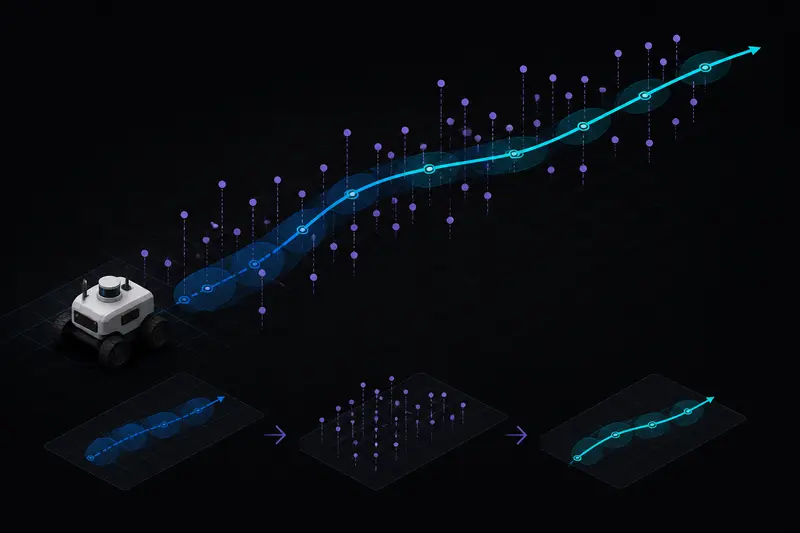
No sensor tells a robot exactly where it is or how fast it is moving. Encoders drift, IMUs accumulate bias, and GPS or vision measurements arrive noisy and sometimes late. A Kalman filter for robot state estimation solves this by combining a mathematical model of how the robot is expected to move with whatever noisy measurements are actually available, producing an estimate that is usually more accurate than either source alone.

This article walks through why that combination works, the core predict-update equations, and a worked 1D example you can extend to a real robot joint or mobile base.

Why Kalman Filter Robot State Estimation Beats Using Sensors Directly

Consider a mobile robot estimating its position along one axis. You have two sources of information: a motion model that predicts the new position from the last known position and commanded velocity, and a sensor (say, a laser rangefinder against a wall) that measures position directly. Neither is trustworthy on its own.

• The motion model drifts over time. Wheel slip, uneven friction, and integration error mean the predicted position wanders further from the truth the longer you rely on it alone.
• The sensor measurement is noisy at any single instant, but it does not drift, since each reading is independent of the last.

The Kalman filter's key insight is that if you know how much you trust each source, expressed as a variance, you can combine them into a single estimate with lower variance, meaning less uncertainty, than either the model prediction or the raw measurement alone. This is the same idea behind weighted averaging: a source you trust more gets more weight.

The Predict-Update Cycle

A Kalman filter runs in a loop of two steps, executed every control cycle:

1. Predict

Using the motion model, project the current state estimate and its uncertainty forward in time, before any new measurement arrives:

x_pred = F * x + B * u
P_pred = F * P * F^T + Q

Here x is the state estimate (for example, position and velocity), F is the state transition matrix describing how the state evolves, B * u accounts for a known control input like commanded velocity, P is the estimate's covariance (uncertainty), and Q is the process noise covariance, how much uncertainty the motion model itself adds each step, from wheel slip, unmodeled friction, and similar effects.

2. Update

When a new measurement z arrives, correct the prediction:

y = z - H * x_pred
K = P_pred * H^T * (H * P_pred * H^T + R)^-1
x = x_pred + K * y
P = (I - K * H) * P_pred

y is the innovation, the gap between what the sensor actually reported and what the model predicted it would report. H maps the state into the space of the measurement (for a direct position sensor, H is often just an identity-like matrix). R is the measurement noise covariance, how noisy the sensor is. K, the Kalman gain, decides how much weight the measurement gets relative to the prediction. When R is large (a noisy sensor), K shrinks and the filter trusts the model more. When Q is large (an unreliable model), K grows and the filter trusts the measurement more.

A Worked 1D Example

Take a simplified case: a robot moving along one axis, state x = [position, velocity], no direct control input for simplicity, sampled every dt seconds.

# State transition: position updates from velocity, velocity assumed constant
F = [[1, dt],
     [0, 1]]

# We only measure position directly
H = [[1, 0]]

# Process noise: uncertainty growth per step from unmodeled dynamics
Q = [[0.001, 0],
     [0, 0.001]]

# Measurement noise: sensor variance, e.g. from a noisy rangefinder
R = [[0.1]]

def predict(x, P):
    x_pred = F @ x
    P_pred = F @ P @ F.T + Q
    return x_pred, P_pred

def update(x_pred, P_pred, z):
    y = z - H @ x_pred
    S = H @ P_pred @ H.T + R
    K = P_pred @ H.T @ inv(S)
    x = x_pred + K @ y
    P = (I - K @ H) @ P_pred
    return x, P

Run predict once per control cycle regardless of whether a measurement arrived, and run update only when a new sensor reading comes in. This is why Kalman filters handle sensors running at different rates gracefully, a wheel encoder at 100 Hz and a camera at 10 Hz can both feed the same filter, each triggering its own update step with its own H and R.

Tuning Q and R

In practice, most of the work in getting a Kalman filter to behave well is tuning Q and R rather than deriving the equations. A few practical guidelines:

• Start by estimating R from real sensor data: log raw measurements while the robot is stationary and compute the variance directly. This gives an honest, data-backed R rather than a guess.
• Q is harder to measure directly. Start small and increase it if the filter lags behind real, sudden changes in the robot's motion, since a too-small Q makes the filter overconfident in a model that can't react quickly.
• If the filter's estimate oscillates or reacts too strongly to individual noisy readings, R is likely too small relative to Q, the filter is trusting each measurement too much.
• If the filter smooths over real motion and lags behind, Q is likely too small relative to R, the filter is trusting the model too much and discounting valid new information.

When You Need an Extended or Unscented Kalman Filter

The standard Kalman filter assumes the state transition and measurement functions are linear, which is rarely exactly true for a robot. A mobile robot's heading-dependent motion model, for instance, involves sine and cosine terms. For these cases, two common extensions exist:

• Extended Kalman Filter (EKF) linearizes the nonlinear functions around the current estimate at each step using a Jacobian, then applies the same predict-update structure. This is the standard choice for mobile robot localization and is well supported in ROS2 packages like robot_localization.
• Unscented Kalman Filter (UKF) avoids linearization entirely by propagating a small set of sample points, called sigma points, through the true nonlinear functions. It tends to handle strong nonlinearity better than an EKF at a modest extra computational cost.

For a robotic arm joint estimating position and velocity from a single encoder, a linear Kalman filter is usually sufficient. Once you are fusing IMU orientation with wheel odometry on a mobile base, an EKF is the more common practical choice. See our IMU sensor fusion basics article for how the same predict-update idea applies specifically to combining accelerometer and gyroscope data.

Where State Estimation Fits in the Control Stack

State estimation and control are separate concerns that feed into each other. A Kalman filter produces the best estimate of position, velocity, or orientation available at each control cycle, and that estimate is what a controller like a PID loop actually uses as its measured value when computing the error against the setpoint. A well-tuned PID controller cannot compensate for a noisy or laggy state estimate feeding it, so getting the estimation stage right upstream tends to pay off more than further PID tuning once the sensor signal itself is the bottleneck.

Summary

A Kalman filter for robot state estimation works by alternating between predicting the next state from a motion model and correcting that prediction with a noisy sensor measurement, weighting each source according to how much you trust it. The core loop, predict then update, is straightforward to implement even in 1D, and the real engineering work is honestly estimating your process noise Q and measurement noise R rather than the matrix algebra itself. For most mobile robots with nonlinear motion models, an Extended or Unscented Kalman Filter extends the same core idea to handle heading and orientation correctly.