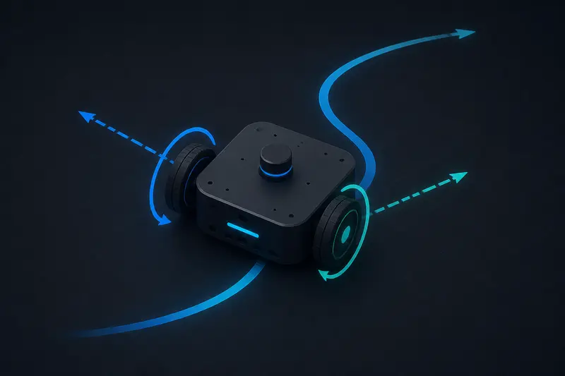
Differential Drive Robot Kinematics and Wheel Odometry: A Worked Example

Differential Drive Robot Kinematics: Why Two Wheels Are Enough to Steer

A differential drive robot has two independently driven wheels on a common axle, usually with one or more passive casters for balance. There's no steering mechanism. Instead, the robot turns by spinning its wheels at different speeds: equal speeds drive straight, unequal speeds curve the path, and opposite speeds spin the robot in place. Differential drive robot kinematics is the math that turns those two wheel speeds into a robot's linear and angular velocity, and the odometry built on top of it is how the robot estimates its own position from nothing but encoder ticks.

This matters for anything from a small research rover to a warehouse AMR: odometry is usually the first position estimate a mobile robot has, often the only one running at full control-loop rate, and it's what other estimators (an EKF, a particle filter, a full SLAM stack) correct against rather than replace outright.

Forward Kinematics: From Wheel Speeds to Robot Velocity

Define two wheels, left and right, separated by a wheelbase (track width) L, each with linear surface speed v_L and v_R (meters per second, computed from wheel radius times angular velocity). The robot's linear velocity v and angular velocity omega at its center point are:

v     = (v_R + v_L) / 2
omega = (v_R - v_L) / L

This is the whole model. When v_R = v_L, omega is zero and the robot drives straight. When v_R = -v_L, v is zero and the robot rotates in place around the midpoint of its axle. Everything else is a mix of forward motion and turning, tracing an arc whose instantaneous radius is R = v / omega (undefined, meaning infinite, when omega is zero).

From Wheel Encoders to Wheel Speed

In practice you don't measure v_L and v_R directly, you measure encoder tick counts and derive them. For a quadrature encoder (see quadrature encoder wiring for the wiring and decoding details), the per-wheel distance traveled between two control loop ticks is:

delta_ticks   = ticks_now - ticks_previous
delta_angle   = 2 * pi * (delta_ticks / counts_per_rev)
delta_distance = delta_angle * wheel_radius

Divide delta_distance by the loop's elapsed time dt to get v_L or v_R for that step. A typical small robot might use a 12 CPR magnetic encoder behind a 30:1 gearbox, giving 360 counts per output wheel revolution, on a 65mm diameter wheel. At a 50Hz control loop, one encoder tick corresponds to roughly 0.57mm of wheel travel, which sets the practical resolution floor of your odometry.

The Discrete Odometry Update

Given v and omega for a short timestep dt, the robot's pose (x, y, theta) updates as:

theta_new = theta + omega * dt
x_new     = x + v * cos(theta) * dt
y_new     = y + v * sin(theta) * dt

This is the standard first-order (Euler) integration used in most real firmware, and it's accurate enough at typical control loop rates (50Hz or faster) where the arc traveled in one step is small. Some implementations use the exact arc-based update instead, which matters more at low update rates or high angular velocity:

if omega != 0:
    x_new     = x + (v/omega) * (sin(theta_new) - sin(theta))
    y_new     = y - (v/omega) * (cos(theta_new) - cos(theta))
    theta_new = theta + omega * dt
else:
    x_new = x + v * cos(theta) * dt
    y_new = y + v * sin(theta) * dt

In Python, a minimal odometry update running inside a control loop looks like this:

def update_odometry(x, y, theta, v_l, v_r, L, dt):
    v = (v_r + v_l) / 2.0
    omega = (v_r - v_l) / L
    theta_new = theta + omega * dt
    x_new = x + v * math.cos(theta) * dt
    y_new = y + v * math.sin(theta) * dt
    return x_new, y_new, theta_new

A Worked Example: How Drift Actually Accumulates

Take a robot with a 0.20m wheelbase, 0.065m wheels, and encoders giving 360 counts per output revolution as above. Command it to drive a 2m straight line at 0.3 m/s, control loop at 50Hz (dt = 0.02s), so 100 steps.

With perfect encoder counts and zero slip, both wheels report identical tick deltas each step, omega stays at zero, and the odometry lands exactly at (2.0, 0.0). Now introduce two realistic error sources:

• Encoder quantization: at 0.57mm resolution per tick, each wheel's measured distance per step can be off by up to half a tick, roughly 0.3mm, in either direction, essentially random noise on each wheel's reported speed.
• Wheel slip asymmetry: a small, consistent difference in effective wheel radius (say the right wheel is 0.3% larger due to tire wear or tire pressure) produces a small but constant nonzero omega even when both wheels are commanded equally.

The encoder quantization noise mostly averages out over many steps since it's symmetric, adding a small random walk to the position estimate, typically a few millimeters of scatter over a 2m run. The wheel radius asymmetry is the more damaging error because it's systematic: a constant 0.3% radius mismatch over a 0.20m wheelbase produces a steady omega of roughly 0.0009 rad/s at 0.3 m/s wheel speed. Integrated over the 6.7 seconds it takes to drive 2m, that's a heading error of about 0.36 degrees, which sounds small but translates to roughly 12mm of lateral position error at the end of the run, and grows linearly with distance traveled. Drive 20m instead of 2m and the same systematic bias produces over 10cm of lateral error.

This is the core lesson of differential drive odometry: random noise sources (encoder quantization, minor timing jitter) mostly average out and grow slowly with the square root of distance, while systematic bias sources (wheel radius mismatch, wheelbase measured incorrectly, gear backlash) grow linearly with distance and dominate over any meaningfully long run.

Calibrating Away the Systematic Error

Two calibration numbers fix most of the systematic drift before it ever reaches a full sensor fusion stage:

1. Effective wheelbase: drive the robot through several full in-place rotations commanded from software, measure the actual rotation with an external reference (a protractor, a floor mark, or an IMU heading reading), and adjust the L used in the kinematics equations until commanded and measured rotation match. The wheelbase that makes the math work is often a few percent different from the physically measured axle distance, because of tire compliance and contact patch effects.
2. Wheel radius ratio: drive a long straight line and measure the actual heading drift. If the robot consistently curves one direction, one wheel's effective radius is slightly larger; apply a small correction factor to that wheel's computed distance per tick until straight-line commands actually drive straight.

These two corrections typically remove the majority of systematic error. What remains, quantization noise and slip during acceleration or on uneven surfaces, is exactly what an IMU sensor fusion layer or a full Kalman filter state estimator is built to correct, by combining odometry with a gyroscope's independent heading estimate and, where available, absolute position fixes.

Common Mistakes

• Using the wrong wheelbase. The geometric axle distance is a starting point, not the value to trust; calibrate it from actual rotation behavior.
• Ignoring gear backlash on direction reversals. A gearbox with play reports encoder motion that doesn't correspond to real wheel motion right after a direction change, corrupting a single step's odometry update.
• Running the odometry update at too low a rate. Euler integration accumulates extra error when omega is large and dt is not small relative to the turn radius; either increase the update rate or switch to the exact arc-based update.
• Treating odometry as ground truth for long-duration autonomy. Odometry alone is fine over short distances, but any mission longer than a few meters needs a correcting sensor layered on top.

Conclusion

Differential drive robot kinematics reduces to two equations connecting wheel speed to linear and angular velocity, and wheel odometry is just integrating that velocity over time using encoder-derived speeds. The forward math is simple enough to implement in a few lines of code, but the real engineering work is understanding which errors are random and self-canceling versus systematic and linearly growing, and calibrating the wheelbase and wheel radius ratio to remove the systematic part before it dominates your position estimate.