Mecanum Wheel Kinematics: A Worked Example from Velocity Command to Wheel Speeds

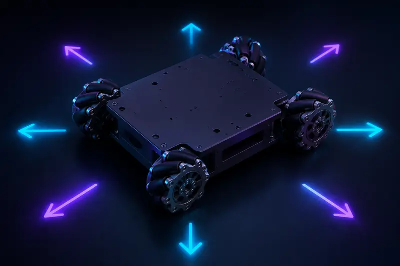
A mecanum drive lets a four wheeled robot translate in any direction while rotating at the same time. The trick is the 45 degree rollers on each wheel rim: each wheel can only push along a diagonal line, and the controller combines four diagonal pushes into the motion you actually want. The math that does this combining is simple matrix arithmetic, but most pages either dump the matrix without numbers or bury it in an academic paper. This article works the whole chain with concrete values: robot geometry in, wheel speeds in rad/s and RPM out.

Mecanum wheel kinematics: setup and conventions

Everything below assumes the standard mounting: looking at the robot from above, the roller axes of the four wheels form an X. If your wheels form an O from above instead, swap the left and right wheel pairs or your robot will rotate when you command a strafe.

Conventions used here:

• x points forward, y points left, positive rotation is counterclockwise (the usual ROS style body frame).
• vx, vy are the commanded body velocities in m/s, wz is the commanded yaw rate in rad/s.
• r is the wheel radius in meters.
• lx is half the front to back wheel spacing, ly is half the left to right wheel spacing, both in meters.

The example robot: 96 mm mecanum wheels (r = 0.048 m), wheel axles 320 mm apart front to back (lx = 0.16 m) and 400 mm apart left to right (ly = 0.20 m). So lx + ly = 0.36 m. That sum acts as the effective lever arm that converts yaw rate into extra wheel speed.

The inverse kinematics equations

Inverse kinematics answers the question you face every control cycle: given a desired (vx, vy, wz), what must each wheel do? For the X configuration the four wheel angular velocities are:

• front left: w_fl = (vx - vy - (lx + ly) * wz) / r
• front right: w_fr = (vx + vy + (lx + ly) * wz) / r
• rear left: w_rl = (vx + vy - (lx + ly) * wz) / r
• rear right: w_rr = (vx - vy + (lx + ly) * wz) / r

Positive wheel speed means the wheel drives the robot forward. Note the pattern: vx appears with the same sign everywhere, vy flips sign between the two diagonals, and the yaw term flips sign between the left and right sides. Those three patterns are the whole secret of mecanum motion.

Case 1: pure forward motion

Command vx = 0.5 m/s, vy = 0, wz = 0. Every equation reduces to 0.5 / 0.048 = 10.42 rad/s, which is about 99.5 RPM. All four wheels spin forward at the same speed and the rollers' side forces cancel. So far the robot behaves exactly like a differential drive.

Case 2: pure strafe

Command vy = 0.5 m/s (strafe left), vx = 0, wz = 0. Now the diagonals split: w_fl = -10.42 rad/s, w_fr = +10.42, w_rl = +10.42, w_rr = -10.42. Front left and rear right spin backward while the other diagonal spins forward. Each wheel pushes along its 45 degree roller line; the forward and backward components cancel and the leftward components add. If your robot pivots instead of strafing when you try this, one wheel is mounted in the wrong orientation or one motor's polarity is flipped.

Case 3: combined motion, the realistic case

Command vx = 0.3 m/s, vy = 0.2 m/s, wz = 0.8 rad/s. First compute the yaw term once: (lx + ly) * wz = 0.36 * 0.8 = 0.288 m/s. Then:

• w_fl = (0.3 - 0.2 - 0.288) / 0.048 = -3.92 rad/s
• w_fr = (0.3 + 0.2 + 0.288) / 0.048 = 16.42 rad/s
• w_rl = (0.3 + 0.2 - 0.288) / 0.048 = 4.42 rad/s
• w_rr = (0.3 - 0.2 + 0.288) / 0.048 = 8.08 rad/s

Four completely different speeds, one of them negative. This is why mecanum drives need per wheel closed loop velocity control: open loop PWM will not hold this ratio as load shifts, and the chassis motion degrades into a smeared arc.

Wheel speed normalization when a motor saturates

Suppose the gearmotors top out at 150 RPM, which is 15.7 rad/s. The front right wheel in case 3 needs 16.42 rad/s (about 157 RPM), slightly beyond the limit. If you just clamp that one wheel, the ratios between wheels break and the robot follows the wrong path. The correct fix is to scale all four wheels by the same factor:

scale = 15.7 / 16.42 = 0.956

The scaled speeds become -3.75, 15.70, 4.23, and 7.72 rad/s. The robot now executes 95.6 percent of the commanded speed along exactly the commanded direction and curvature. Direction is preserved, magnitude is sacrificed. Every serious mecanum implementation does this.

Forward kinematics for odometry

Running the equations the other way turns measured wheel speeds into body velocity, which you integrate for odometry:

• vx = (r / 4) * (w_fl + w_fr + w_rl + w_rr)
• vy = (r / 4) * (-w_fl + w_fr + w_rl - w_rr)
• wz = (r / (4 * (lx + ly))) * (-w_fl + w_fr - w_rl + w_rr)

The wheel speeds come from your encoders, and the quality of that measurement matters more here than on a differential drive because four noisy estimates get combined. The techniques in robot joint velocity estimation from encoder counts apply directly to mecanum wheel encoders.

A compact Python implementation

def mecanum_ik(vx, vy, wz, r=0.048, lx=0.16, ly=0.20, w_max=15.7):
    k = (lx + ly) * wz
    w = [(vx - vy - k) / r,   # front left
         (vx + vy + k) / r,   # front right
         (vx + vy - k) / r,   # rear left
         (vx - vy + k) / r]   # rear right
    peak = max(abs(s) for s in w)
    if peak > w_max:
        w = [s * w_max / peak for s in w]
    return w

Feed the returned values as setpoints to four independent wheel velocity loops. Do not skip the normalization branch; it is two lines and it is the difference between a robot that tracks its path at high command levels and one that veers.

Why strafing is worse than the math suggests

The mecanum wheel kinematics above are exact for ideal wheels, but three real world effects hit sideways motion hardest:

• Roller losses. When strafing, all the drive force passes through rollers spinning on their own small bearings. Friction there wastes torque and the robot strafes noticeably slower than it drives forward for the same wheel speed.
• Weight distribution. The force balance only cancels correctly if all four wheels carry comparable load. A nose heavy robot yaws while strafing because the lightly loaded rear wheels slip first. Check this before touching software: push the robot sideways slowly and watch which corner skids.
• Odometry drift in y. Roller slip means integrated vy is the least trustworthy odometry channel. Fuse a gyro for heading at minimum, and treat lateral position from wheel odometry as a rough estimate, the same lesson covered for two wheeled robots in differential drive kinematics and wheel odometry, only worse.

Rule of thumb: trust mecanum odometry in x about as much as differential drive odometry, trust wz only with a gyro, and trust y the least. Plan your localization stack around that ranking.

Checklist for a first bring up

1. Verify the X roller pattern from above and correct motor polarity so positive command drives every wheel forward.
2. Measure r, lx, ly with calipers and a tape measure; a 5 percent radius error is a 5 percent velocity error on every command.
3. Command pure vx, then pure vy, then pure wz, and confirm each produces only the intended motion.
4. Add the normalization scaling before you ever command combined motion near full speed.
5. Close a velocity loop on each wheel before trusting the chassis level behavior.

Work through those five steps with the equations above and a mecanum base becomes a predictable, controllable platform instead of a drifting mystery.