Robot Joint Velocity Estimation from Encoder Counts: Why Finite Differences Get Noisy

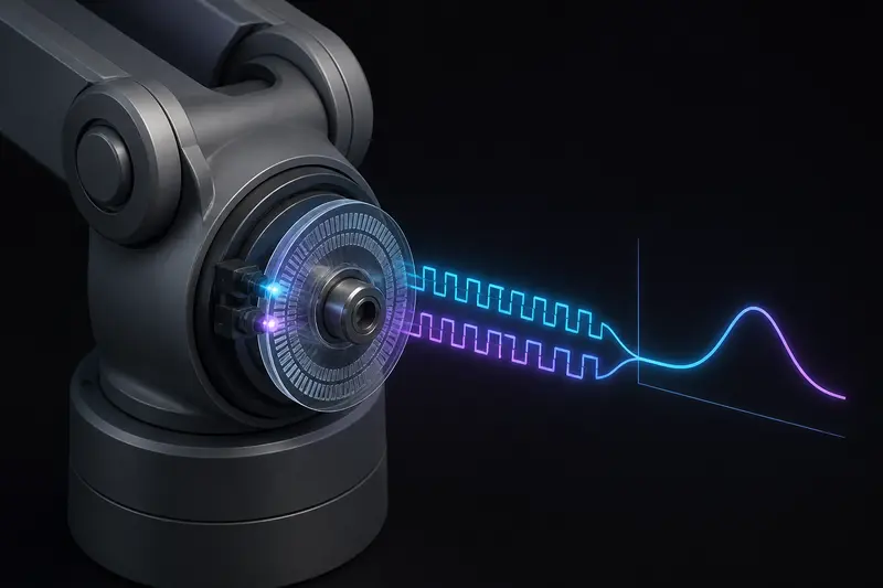
Almost every robot joint controller needs a velocity signal: the damping term in a PD position loop, the feedback for a cascaded velocity loop, the friction model input. Almost no hobby or research arm has a tachometer, so that velocity has to be computed from the position encoder. The obvious approach, subtracting two consecutive positions and dividing by the sample time, produces a signal so noisy that many builders assume their encoder is broken. It is not. The noise is baked into the arithmetic, and once you see the numbers you also see the fixes.

Why Robot Joint Velocity Estimation from Encoder Counts Is Hard

Take a common setup: a 2048-line incremental encoder read in quadrature, so 8192 counts per revolution, sampled by a 1 kHz control loop. One count corresponds to:

delta_theta = 2*pi / 8192 = 7.67e-4 rad = 0.044 deg

The finite difference estimate is omega = (theta[k] - theta[k-1]) / dt. With dt = 0.001 s, the smallest nonzero velocity this can report is one count per sample:

omega_step = 7.67e-4 rad / 0.001 s = 0.767 rad/s = 44 deg/s

That is the entire problem in one number. The estimator cannot output anything between 0 and 44 deg/s. Now let the joint move at a realistic tracking speed of 10 deg/s (0.175 rad/s). The encoder delivers about 227 counts per second, which is 0.23 counts per 1 ms sample. So roughly three out of four samples report zero velocity, and one out of four reports 44 deg/s. The true signal is a steady 10 deg/s; the raw finite difference is a square-ish wave slamming between 0 and 44. Feed that into a derivative or velocity gain and the motor current buzzes audibly.

Note that this is quantization noise, not electrical noise. A perfect encoder and a perfect counter still produce it. Robot joint velocity estimation is therefore a filtering problem from the start, and every practical method below trades noise against delay in a different way.

Method 1: Widen the Difference Window

Instead of differencing adjacent samples, difference over N samples: omega = (theta[k] - theta[k-N]) / (N*dt). The one-count step shrinks by N, the delay grows with N. For N = 16 at 1 kHz:

• Velocity resolution: 0.767 / 16 = 0.048 rad/s = 2.7 deg/s
• Effective delay: about (N-1)/2 samples = 7.5 ms

That resolution is usable for a modest position loop, and 7.5 ms of lag is tolerable if your velocity loop bandwidth is 10 Hz or below. Push the loop bandwidth toward 50 Hz and that lag starts eating your phase margin. The window method is the right first step because it is two lines of code and completely predictable.

Method 2: Low-Pass Filtered Derivative

The classic dirty derivative runs the raw finite difference through a first-order low-pass filter:

omega_f[k] = a * omega_f[k-1] + (1 - a) * omega_raw[k]

with a = exp(-2*pi*fc*dt). For a 25 Hz cutoff at 1 kHz, a = 0.855. The filter time constant is 1/(2*pi*25) = 6.4 ms, so the lag is comparable to the N = 16 window, and the count noise standard deviation drops by roughly a factor of 3 to 4 for this cutoff. The advantage over the window is that you tune one intuitive parameter, the cutoff frequency, and you can place it just above your loop bandwidth. The disadvantage is the long exponential tail: after a step change in speed the estimate creeps toward the true value instead of arriving at a known fixed delay.

Method 3: Measure Time Between Counts (1/T Method)

The first two methods count edges per fixed time. At low speed it is far better to invert the measurement: timestamp each encoder edge with a hardware timer and compute omega = delta_theta / T, where T is the measured interval between counts. Most microcontroller timers capture edges with 1 us resolution or better.

At our 10 deg/s example the interval between counts is 1/227.5 s = 4396 us. A plus or minus 1 us capture error gives a velocity error of about 0.02 percent. Compare that with the 440 percent relative steps of the raw finite difference at the same speed. This is why servo drive firmware almost universally uses edge timing at low speed.

The catch is high speed. At a motor-side speed of 3000 rpm the same encoder produces 409,600 counts per second, the interval shrinks to 2.4 us, and the same 1 us capture uncertainty is now a 40 percent error, assuming your interrupt handler even survives 400k events per second (it will not; you must use hardware capture and decimation). Real implementations switch between edge timing at low speed and counts-per-period at high speed, or use the combined M/T method that measures both counts and time over each window.

Method 4: A Tracking Loop Observer

The cleanest general-purpose solution is a small observer, essentially a software PLL, that integrates an estimated velocity into an estimated position and steers both with the position error:

err = theta_meas - theta_hat
omega_hat += Ki * err * dt
theta_hat += (omega_hat + Kp * err) * dt

Because the velocity state is reached through an integrator, the output is smooth by construction, and because the loop has two integrations it tracks a constant velocity with zero steady-state lag, something none of the previous methods can claim. Tune it like a second-order system: pick a natural frequency omega_n and damping ratio zeta = 1, then Kp = 2*zeta*omega_n and Ki = omega_n squared. For omega_n = 2*pi*25 rad/s that gives Kp = 314 and Ki = 24674. Raise omega_n for faster tracking, lower it for more smoothing. If you know the commanded motor torque you can add it as a feedforward acceleration into omega_hat, which turns this into a simple Luenberger observer and improves response during transients.

Which Method Should You Use?

• Quick prototype, loop bandwidth under 10 Hz: windowed finite difference, N sized so the velocity resolution is under about 10 percent of your typical speed.
• Standard PD or cascaded loop: tracking loop observer at 3 to 5 times your intended velocity loop bandwidth. It is 5 lines of code and behaves better than any fixed filter.
• Very low speeds or heavy gearing: hardware edge timing (1/T or M/T) if your timer peripheral supports capture; it is the only method that stays accurate near zero speed.
• Persistent noise despite all this: check the encoder itself. Electrical noise on the A/B lines creates false counts that no estimator can remove; see our guide on quadrature encoder wiring for a 6-DOF arm for the signal-integrity side.

Conclusion

Robot joint velocity estimation fails in a very predictable way: the one-count velocity step, delta_theta / dt, is often larger than the velocity you are trying to measure. Compute that number for your encoder and loop rate before writing any filter code. If it is small compared to your working speeds, a windowed difference is fine. If not, use a tracking loop observer, or move the measurement into hardware with edge timing. And if the step size itself is the bottleneck, the real fix is mechanical: more counts per revolution, chosen the same way as in our article on sizing encoder resolution for robot joints, where velocity ripple sets the resolution floor long before position accuracy does.