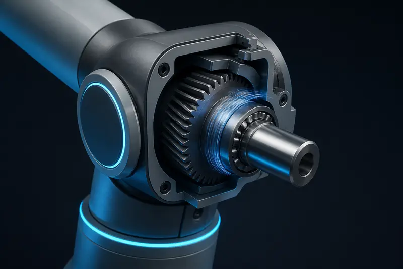
Why robot arm joint friction compensation matters
If a joint moves smoothly at high speed but jitters, sticks, or stalls entirely near zero velocity, the problem is almost never your PD or PID gains. It is friction. Every geared robot joint has static friction (stiction) that must be overcome before motion starts, and once moving, a velocity-dependent drag that keeps opposing the motor. Robot arm joint friction compensation adds a feedforward torque term that cancels this drag directly, instead of asking the feedback loop to fight it with error alone.
This matters most at low speed. A well-tuned position loop can look perfect during a fast trajectory and still buzz or stall when the arm is asked to creep slowly toward a target, because the required corrective torque near zero velocity is dominated by friction, not inertia.
The two friction terms you can actually model
A practical friction model for a hobby or small industrial joint has two additive terms:
- Coulomb friction (
tau_c): a constant-magnitude torque that opposes motion, independent of speed. It comes from dry contact between gear teeth, bearings, and seals. - Viscous friction (
b): a torque proportional to velocity, from lubricant drag and cabling resistance.
Combined, the friction torque as a function of joint velocity qdot is:
tau_friction(qdot) = tau_c * sign(qdot) + b * qdot
This ignores the Stribeck effect (the extra drop in friction right around zero velocity as a joint transitions from static to kinetic friction). That refinement matters for high-precision industrial joints, but the two-term model above already removes most of the stick-slip behavior a hobby or small-arm builder will see, and it only needs one simple test to identify.
A note on sign(qdot) at zero velocity
The sign function is undefined at exactly zero velocity, and a naive implementation will chatter between +tau_c and -tau_c when the joint is nominally at rest. In practice, clamp the Coulomb term to zero (or to a small linear ramp) inside a narrow velocity deadband, typically a few encoder counts per control cycle, so the compensator does not inject torque noise when the joint is genuinely holding still.
Measuring the coefficients: a constant-velocity test
You do not need a dynamometer to get usable numbers. With the arm oriented so gravity torque on the joint is zero or already compensated (see our gravity compensation article for that separate term), command the joint to move at a series of constant velocities in open loop or under velocity control, and log the steady-state torque (from current sensing, as in our torque control article) required to hold each speed.
Suppose you run the joint at five target speeds and record the following steady-state torques, with each speed run in both directions and averaged to cancel any residual gravity offset:
| qdot (rad/s) | Measured torque (N*m) |
|---|---|
| 0.10 | 0.084 |
| 0.30 | 0.098 |
| 0.60 | 0.119 |
| 1.00 | 0.146 |
| 1.50 | 0.181 |
Since tau = tau_c + b * qdot for qdot > 0, this is a straight line. Fit it with a simple linear regression (least squares on the five points above):
b = 0.0655 N*m*s/rad
tau_c = 0.077 N*m
You can sanity-check the fit by hand: between qdot = 0.10 and qdot = 1.50, torque rose by 0.181 - 0.084 = 0.097 N*m over a velocity change of 1.40 rad/s, giving b = 0.097 / 1.40 = 0.069 N*m*s/rad, close to the regression value. The intercept, torque extrapolated back to qdot = 0, gives tau_c directly.
Adding the feedforward term to your control loop
With tau_c and b identified, the compensator sits alongside your existing PD or PID position loop and any gravity feedforward term:
tau_cmd = Kp*(q_des - q) + Kd*(qdot_des - qdot) + tau_gravity(q) + tau_c*sign(qdot_des) + b*qdot_des
Using the desired velocity qdot_des from the trajectory rather than the measured qdot is a deliberate choice: it avoids amplifying encoder velocity noise into the friction term, and it lets the compensator anticipate the friction the joint is about to experience rather than reacting after the fact. Pseudo-code for one control cycle:
def friction_feedforward(qdot_des, tau_c, b, deadband=0.02):
if abs(qdot_des) < deadband:
coulomb_term = tau_c * (qdot_des / deadband)
else:
coulomb_term = tau_c * sign(qdot_des)
return coulomb_term + b * qdot_des
The linear ramp inside the deadband avoids the chatter problem mentioned earlier while still applying most of the breakaway torque as the joint starts to move.
Diagnosing under- or over-compensation
Three symptoms tell you which direction to adjust the fitted coefficients:
- Stick-slip jitter during slow, continuous motion. The joint moves in small jumps instead of a smooth creep. This is under-compensated Coulomb friction: the feedforward torque is not enough to fully overcome breakaway friction, so the PD loop has to build up error before the joint releases.
- Overshoot or a slight buzz right as the joint starts moving from rest. This is over-compensated Coulomb friction, usually from measuring tau_c on a joint that was partially loaded by gravity during the test. Re-run the constant-velocity test with the arm balanced or with gravity compensation active.
- Steady-state tracking error that grows with commanded speed. This points at an underestimated viscous coefficient b. Add another data point at a higher velocity and refit.
A joint that only ever moves at moderate-to-high speed may not need this term at all, since a PD loop with reasonable gains can often absorb constant-magnitude drag through steady-state error. Friction compensation earns its complexity specifically at low speed and near direction reversals, which is exactly where uncompensated joints look worst in a trajectory-following or force-control task.
Building or studying robotics?
Arcbotix publishes practical guides on robotics engineering, control systems and real-world builds. Explore more articles on the blog.