Robot Arm Singularity Avoidance with the Jacobian: A Worked Example

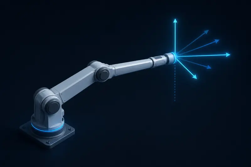
A robot arm singularity is a joint configuration where the arm momentarily loses the ability to move its end effector in some direction, no matter how the joints are commanded. Robot arm singularity avoidance matters because a controller that does not detect these poses in advance can command joint velocities that spike toward infinity, causing violent, unpredictable motion. This article walks through detecting a singularity with the Jacobian determinant on a concrete two-link arm, then compares two practical ways to keep the controller stable when the arm gets close to one.

What a Singularity Actually Is

For a serial manipulator, the Jacobian matrix J relates joint velocities to end-effector velocity:

v = J(q) * q_dot

where q is the vector of joint angles, q_dot is joint velocity, and v is the end-effector's linear (and angular, for 6-DOF arms) velocity. To move the end effector at some desired velocity, the controller inverts this relationship:

q_dot = J^-1(q) * v

As covered in inverse kinematics explained, this pseudo-inverse relationship is also how iterative IK solvers work. This works fine as long as J is invertible. At a singularity, J loses rank: its determinant goes to zero, J^-1 blows up, and the same small end-effector velocity command demands infinite joint velocity. Physically, this happens when two or more joint axes line up so that moving either one produces the same effect on the end effector, or when the arm is fully stretched out and has no remaining reach in the outward direction.

Robot Arm Singularity Avoidance: A 2-Link Worked Example

Take a planar 2-link arm with link lengths L1 and L2, joint angles theta1 and theta2 (theta2 measured relative to link 1). The end-effector position is:

x = L1*cos(theta1) + L2*cos(theta1+theta2)
y = L1*sin(theta1) + L2*sin(theta1+theta2)

Differentiating gives the 2x2 Jacobian:

J = [ -L1*sin(theta1)-L2*sin(theta1+theta2), -L2*sin(theta1+theta2) ;
 L1*cos(theta1)+L2*cos(theta1+theta2),  L2*cos(theta1+theta2) ]

Its determinant simplifies to a clean expression:

det(J) = L1 * L2 * sin(theta2)

This is the entire story for a 2-link arm: det(J) is zero whenever theta2 is 0 or 180 degrees. theta2 = 0 means the arm is fully extended (both links pointing the same direction) - the classic outstretched singularity. theta2 = 180 degrees means the arm is folded back on itself, which is a less common but equally real singular pose.

Plugging in Numbers

With L1 = 0.3 m and L2 = 0.25 m, here is det(J) at a few elbow angles:

• theta2 = 90 deg: det(J) = 0.3 * 0.25 * sin(90) = 0.075
• theta2 = 30 deg: det(J) = 0.3 * 0.25 * sin(30) = 0.0375
• theta2 = 10 deg: det(J) = 0.3 * 0.25 * sin(10) = 0.013
• theta2 = 1 deg: det(J) = 0.3 * 0.25 * sin(1) = 0.0013
• theta2 = 0 deg: det(J) = 0 (singular)

Now suppose the controller commands an end-effector velocity of 0.1 m/s outward, and it solves q_dot = J^-1 * v directly. Because J^-1 scales roughly with 1/det(J), the required joint velocity climbs sharply as theta2 shrinks: it is manageable at 90 degrees, already uncomfortable at 10 degrees, and effectively unbounded by 1 degree. A real servo or gearbox cannot deliver that, so the arm either stalls, trips a current limit, or (worse) briefly tries to comply and jerks.

Detecting the Problem: Manipulability, Not Just det(J) = 0

Checking det(J) == 0 exactly is fragile in floating point and only tells you about exact singularities, not near-singular poses where the same blow-up already starts. A more useful signal is Yoshikawa's manipulability measure:

w = sqrt(det(J * J^T))

For a square, non-redundant Jacobian this reduces to abs(det(J)). The practical use is a threshold check the controller runs every cycle: if w drops below some fraction of its typical working-region value (a common starting point is 5-10% of the manipulability at a well-conditioned reference pose), treat the arm as near-singular and switch behavior before the joint velocities actually spike.

Two Ways to Handle It in the Controller

1. Plain Pseudo-Inverse (What Breaks)

For redundant or non-square Jacobians, the Moore-Penrose pseudo-inverse J+ = J^T * (J * J^T)^-1 is the standard way to solve q_dot = J+ * v. The problem is that J * J^T is exactly what goes singular in the same poses, so the pseudo-inverse inherits the same blow-up. It is not a fix by itself, just a more general way to write the same fragile inversion.

2. Damped Least Squares (What Actually Helps)

Damped least squares (DLS), sometimes called the Levenberg-Marquardt method in this context, adds a small damping term lambda to trade a bounded amount of tracking error for bounded joint velocity:

q_dot = J^T * (J * J^T + lambda^2 * I)^-1 * v

With lambda = 0, this is identical to the plain pseudo-inverse. As lambda increases, the joint velocity solution stays finite even as det(J) approaches zero, at the cost of the end effector tracking the commanded velocity less exactly near the singularity. A practical scheme makes lambda adaptive: near zero when manipulability w is healthy (so tracking stays exact in the normal working volume), and ramping up smoothly as w drops below the threshold from the manipulability check above.

Continuing the 2-link example at theta2 = 1 degree, a fixed damping of lambda = 0.02 keeps the effective denominator away from zero, capping joint velocity to a sane range instead of the near-infinite value the plain inverse would demand, at the cost of a small, boundable deviation from the requested 0.1 m/s end-effector path right at that instant.

Practical Guidelines

• Compute manipulability w every control cycle, not just det(J); it is cheap (one 2x2 or 3x3 determinant for most arm sizes) and catches near-singular poses before they become exact ones.
• Set the damping threshold from your own arm's healthy-pose manipulability, not a generic constant - a small desktop arm and a heavy industrial arm have very different natural magnitudes for w.
• Prefer trajectory planning that keeps the arm's elbow away from full extension and full fold-back when the task allows it, rather than relying on damping alone to save every pose; damping trades accuracy for safety, it does not remove the underlying geometric problem. This is also a good reason to check reachable poses during the planning stage described in trajectory planning for robotic arms, rather than only reacting to singularities at execution time.
• Log the damping factor lambda actually applied during operation. If it is frequently non-zero in normal use, that is a sign the workspace or task path is routing too close to a singular region and the trajectory, not just the controller, needs adjusting.

Why This Matters Beyond the Math

Singularities are not an edge case reserved for redundant or exotic arm designs. Any serial arm with two or more links has at least a full-extension singularity, and most reachable workspaces include poses close enough to it that naive inverse kinematics solvers will occasionally hand back an unreasonable joint velocity command. Robot arm singularity avoidance is really two separate habits: detecting proximity to a singularity with a cheap manipulability check, and using damped least squares (or an equivalent bounded-velocity method) so the controller degrades gracefully instead of demanding motion the hardware cannot deliver.