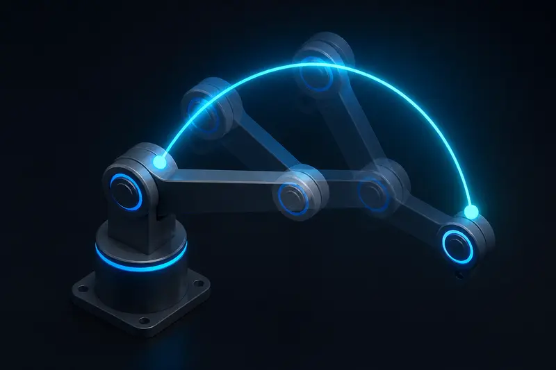
Trajectory Planning for Robotic Arms: From Waypoints to Smooth Motion

Trajectory planning for robotic arms is the step between knowing where a joint needs to end up and actually commanding it to move there. An inverse kinematics solver or a motion planner gives you a target pose. On its own, that target is useless to a real actuator: you cannot simply tell a motor "go to 47 degrees" and expect smooth, safe motion. Something has to generate the full time-parameterized path, position, velocity, and acceleration at every control cycle, between where the joint is now and where it needs to be.

This article covers the two main planning spaces, the velocity profiles used to keep motion smooth, and the practical failure modes that show up when trajectory planning is done poorly.

What Trajectory Planning Actually Produces

A trajectory is not just a path. A path is a set of geometric points in space. A trajectory adds the time dimension: it specifies position, velocity, and acceleration as continuous functions of time, sampled at the controller's update rate (often 100 Hz to 1 kHz depending on the platform).

For a single joint moving from angle q0 to q1, the planner must produce a function q(t) such that:

• q(0) = q0 and q(T) = q1
• Velocity starts and ends at zero (or matches a specified boundary condition)
• Velocity and acceleration never exceed the actuator's physical limits
• The resulting motion is continuous enough that the joint's PID or torque controller can actually track it

This last point matters more than it sounds. A trajectory that jumps in velocity or acceleration creates a tracking error spike that a well-tuned PID controller will fight against, often producing overshoot or audible motor strain.

Joint Space vs Cartesian Space Planning

There are two fundamentally different places to plan a trajectory: in joint space or in Cartesian (task) space.

Joint Space Trajectories

In joint space planning, you compute a separate time-parameterized trajectory for each joint independently, then run them concurrently so all joints start and finish at the same time. This is the simpler and more common approach for point-to-point moves.

Advantages:

• No singularities: joint space has no configuration where the math breaks down, unlike Cartesian space near a wrist singularity
• Computationally cheap: each joint is planned independently with simple closed-form profiles
• Naturally respects joint velocity and acceleration limits, since you plan directly in those units

Disadvantage: the end effector's path through 3D space is not controlled directly. Moving from one pose to another in joint space can cause the end effector to sweep through an unexpected arc, which is a problem if there is an obstacle or a table surface in the way.

Cartesian Space Trajectories

Here you plan the end effector's position and orientation directly, for example a straight line from point A to point B, then use an inverse kinematics solver at each timestep to convert the desired Cartesian pose back into joint angles.

This is necessary whenever the path itself matters, welding a straight seam, drawing a line, moving through a narrow gap, but it is more expensive and can run into two problems: IK solutions that vary discontinuously between nearby poses, and singularities where a small Cartesian motion requires an infinite joint velocity.

A practical rule: use joint space planning for free-space point-to-point moves, and switch to Cartesian planning only when the task genuinely requires control over the end effector's path shape.

Velocity Profiles: Trapezoidal and S-Curve

Once you know the space you are planning in, you need a profile that defines how velocity changes over time during the move. Two profiles dominate industrial and hobbyist robotics.

Trapezoidal Velocity Profile

The trapezoidal profile is the default choice for most point-to-point moves. It has three phases:

1. Acceleration phase: constant acceleration from zero to a cruise velocity
2. Constant velocity phase: cruise at maximum allowed velocity
3. Deceleration phase: constant deceleration back to zero

Plotted, velocity over time looks like a trapezoid, hence the name. For a move of distance d with maximum velocity v_max and maximum acceleration a_max, the time to reach cruise velocity is t_acc = v_max / a_max. If the distance covered during acceleration and deceleration exceeds d, the profile becomes triangular instead, meaning the joint never reaches v_max before it must start decelerating.

The trapezoidal profile is simple to compute and respects hard velocity and acceleration limits, but it has a discontinuous acceleration: at the transition from acceleration to cruise, acceleration jumps instantly from a_max to zero. That instantaneous jump is what causes the physical jerk (rate of change of acceleration) that shows up as a small shudder in real hardware.

S-Curve Velocity Profile

An S-curve profile adds a jerk-limited ramp to both the acceleration and deceleration phases, so acceleration itself changes smoothly instead of jumping. Instead of three phases, there are seven: jerk up, constant acceleration, jerk down, cruise, jerk down (into deceleration), constant deceleration, jerk up (back to zero).

The tradeoff is straightforward: S-curves take slightly longer to execute the same move because ramping acceleration smoothly costs time, but they produce noticeably smoother motion, less mechanical wear, and lower peak torque demand on the motor. For arms handling fragile payloads, or with backlash-prone gearboxes such as those discussed when comparing harmonic drives to planetary gearboxes, the reduction in jerk is often worth the small time penalty.

A rough heuristic: if your arm makes an audible clunk or visible shudder at the start or end of a move, you are almost certainly running a trapezoidal profile and hitting its acceleration discontinuity. Switching to an S-curve or a quintic polynomial blend usually fixes it without touching the PID gains at all.

Polynomial Trajectories

An alternative to piecewise velocity profiles is fitting a single polynomial to the whole move. A cubic polynomial q(t) = a0 + a1*t + a2*t^2 + a3*t^3 can satisfy position and velocity boundary conditions at both ends (four constraints, four coefficients). A quintic (5th-order) polynomial adds two more coefficients, letting you also specify acceleration at the start and end, which is what you want for smoothly chaining multiple trajectory segments together without a velocity or acceleration discontinuity at the boundary.

Quintic polynomials are common in academic robotics and in multi-segment trajectories where several waypoints must be visited without stopping at each one. The cost is that peak velocity and acceleration are harder to bound directly since they are a byproduct of the polynomial coefficients rather than a planned parameter, so you typically compute the polynomial first and then verify it does not exceed actuator limits.

Multi-Joint Synchronization

When multiple joints move at once, each joint has its own maximum velocity and acceleration, and its own distance to travel. If you plan each joint at its own maximum speed, the joints will finish at different times, and the end effector's path becomes unpredictable.

The standard fix is time scaling: compute the minimum time each joint would need at its own limits, take the slowest joint as the limiting factor, then scale down every other joint's trajectory to match that same total duration. All joints start and stop together, and the one that was already going to take the longest sets the pace for the whole move.

Practical Checklist

• Plan in joint space for free-space moves, Cartesian space only when the path shape matters
• Use trapezoidal profiles as a fast default, switch to S-curve or quintic polynomials if you see jerk-related vibration or wear
• Always scale multi-joint trajectories to a common duration set by the slowest joint
• Verify computed peak velocity and acceleration against actuator datasheet limits before deploying, especially for polynomial-based trajectories
• Re-check trajectories whenever payload changes, since added mass reduces the safe acceleration limit for a given motor

Summary

Trajectory planning for robotic arms turns a start and end configuration into a smooth, time-parameterized motion that the joint controllers can actually track. Joint space planning is simpler and avoids singularities; Cartesian planning is necessary when the end effector's path matters. Trapezoidal profiles are the practical default, while S-curve and quintic polynomial profiles trade a small amount of execution time for significantly smoother, lower-jerk motion. Getting this layer right often solves motion quality problems that look like they need PID retuning but are actually caused by a discontinuous trajectory feeding the controller a signal it cannot follow cleanly.